Day 20-Machine Learning

🌟 Concept Overview

Gradient Boosting is a sequential ensemble technique — unlike Random Forest (parallel bagging), each model learns from the errors (residuals) of the previous one.
You’re using simple decision stumps (tiny trees) as weak learners, gradually improving predictions

---

🧮 Key Formulas

• Loss function:

\(L = \frac{1}{2}(y - \hat{y})^2 \)

• Gradient (negative direction):

\(-g = y - F \)

• Model update rule:

\(F_m(x) = F_{m-1}(x) + \eta \cdot h_m(x) \)

---

🧩 Step 0 — Initial Model F0

• Start with a constant prediction F0=mean(y)=154.

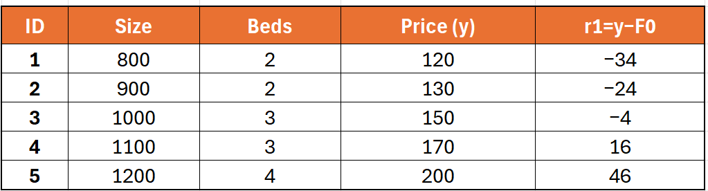
• Compute residuals r1=y−F0.
  These residuals become the targets for the first stump.

Dataset:

\(F_0 = \text{mean}(y) = \frac{120 + 130 + 150 + 170 + 200}{5} = 154 \)

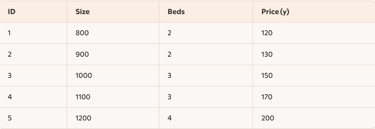
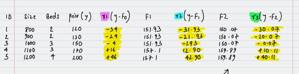
Residuals r1=y−F0:

These residuals become the targets for the first stump.

---

🧮 Step 1 — Candidate Splits for h₁(x)

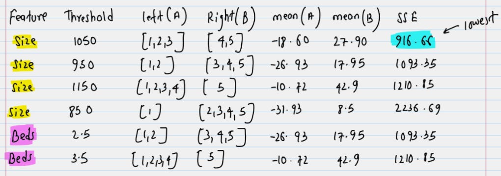
• Candidate splits tested on Size and Beds.

• For each threshold, compute mean residuals on left/right and SSE (sum of squared errors).

• The best split (lowest SSE = 916.66) is Size < 1050.

  • Left mean = −20.66, Right mean = 31.

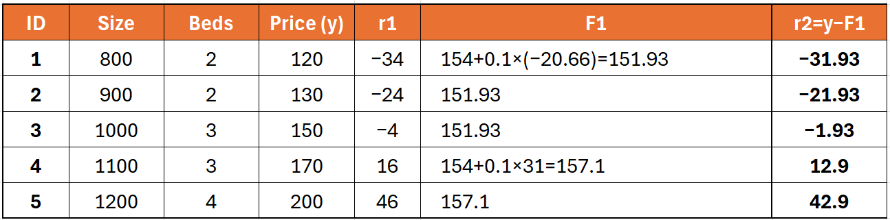
• Update model: F₁(x)=F₀+η⋅h1(x)

where learning rate η=0.1.

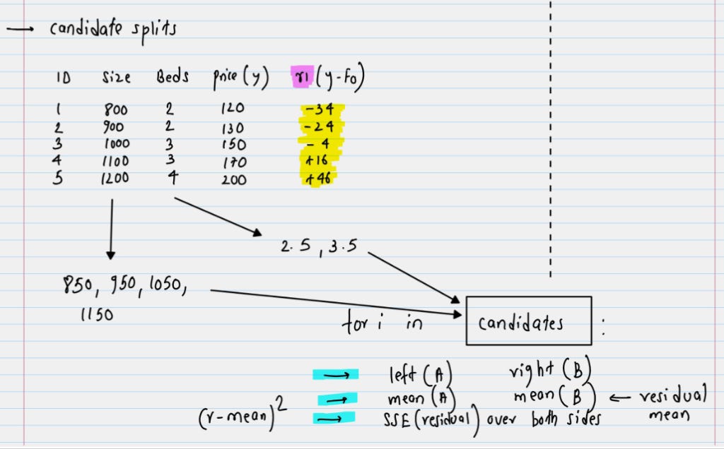
🌳 Candidate Splits — Definition

When training a tree (or stump in boosting), the algorithm must decide where to split the data.

• A candidate split is simply a possible threshold on a feature.

• Example:

  • Feature = Size

  • Candidate splits = 850, 900, 950, 1000, 1050, etc.

  • Each split divides the dataset into Left group (values ≤ threshold) and Right group (values > threshold).

The algorithm evaluates all candidate splits across all features, then chooses the one that minimizes error (variance, SSE, Gini, entropy, depending on the task).

---

we calculate for all the mid points i.e. for both the features size and beds i.e. 850, 950, 1050, 1150 and for Beds it will be 2.5 and 3.5

Below is the calculation for the same

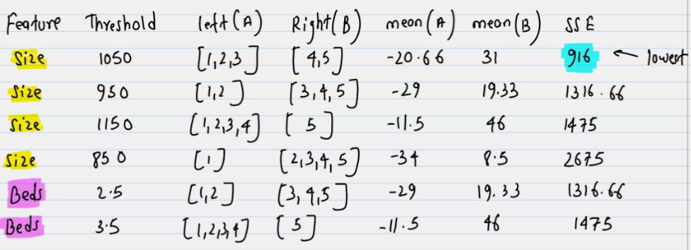
Let us take the Threshold of 1050 and break up of all the calculation as follows and the same calculation applies for all other threshold to that 950,1150,850,2.5, 3.5 and we select the lowest SSE

---

Example: Size < 1050

Left = [1, 2, 3], Right = [4, 5]

Left residuals: [−34, −24, −4]
Right residuals: [16, 46]

\(\begin{aligned} \text{mean}(A) &= \frac{-34 - 24 - 4}{3} = -20.66 \\[2ex] \text{mean}(B) &= \frac{16 + 46}{2} = 31 \end{aligned} \)

Now compute SSE for each side:

Formula

\(\text{SSE} = \sum_{i=1}^{n} (y_i - \hat{y}_i)^2 \)

Left (A)

with each residual value we are multiplying the Mean of A

\(\begin{aligned} (-34 - (-20.66))^2 &= (-13.33)^2 = 177.7 \\[1.5ex] (-24 - (-20.66))^2 &= (-3.33)^2 = 11.1 \\[1.5ex] (-4 - (-20.66))^2 &= (16.66)^2 = 277.7 \\[2.5ex] \text{SSE}(A) &= 177.7 + 11.1 + 277.7 = 466.5 \end{aligned} \)

Right (B)

with each residual value we are multiplying the Mean of B

\(\begin{aligned} (16 - 31)^2 &= (-15)^2 = 225 \\[1.5ex] (46 - 31)^2 &= (15)^2 = 225 \\[2.5ex] \text{SSE}(B) &= 225 + 225 = 450 \end{aligned} \)

\(\begin{aligned} \mathbf{\text{Total SSE}} &\mathbf{= 466.5 + 450 = 916.5} \end{aligned} \)

✅ Lowest SSE = 916.5 → Best split: Size < 1050

---

🌳 Step 2 — First Stump h₁(x)

We started with the initial model prediction

• F₀=154.

• Residuals r1=y−F₀:

Now, from the above steps we understood the Best split: Size < 1050

Candidate Split: Size < 1050

This split divides the data into:

• Left group (Size < 1050): Id’s 1, 2, 3 → residuals [−34, −24, −4]

• Right group (Size ≥ 1050): Id’s 4, 5 → residuals [+16, +46]

🔢 Left Group Mean

\(\begin{aligned} \text{mean}(A) &= \frac{-34 + (-24) + (-4)}{3} \\[1.5ex] &= \frac{-62}{3} = -20.66 \end{aligned} \)

🔢 Right Group Mean

\(\begin{aligned} \text{mean}(B) &= \frac{16 + 46}{2} \\[1.5ex] &= \frac{62}{2} = 31 \end{aligned} \)

📌 Interpretation

• For any house with Size < 1050, the stump predicts the average residual of that group: −20.66.

• For any house with Size ≥ 1050, the stump predicts the average residual of that group: +31.

That’s why the stump is written as:

\(h_1(x) = \begin{cases} -20.66 & \text{if } \text{Size} < 1050 \\[1ex] 31 & \text{otherwise} \end{cases} \)

✅ Why This Split Was Chosen

We tested multiple candidate splits (Size < 850, Size < 950, Beds < 3, etc.).
For each, we computed the Sum of Squared Errors (SSE).

• Size < 1050 gave the lowest total SSE (≈ 916.5).

• That’s why it was selected as the first stump.

👉 So the “−20.66” and “31” are simply the average residuals of the two groups formed by the split at 1050.

---

Learning rate η=0.1

Update model:

F₀ =154 from previous steps

\(F_1(x) = F_0 + \eta \cdot h_1(x) \)

---

🧮 Step 3 — Second Stump h₂(x)

Now fit a new stump on residuals r₂.

Candidate splits again tested on Size and Beds.
Best split still Size < 1050 (lowest SSE = 916.6).

Left residuals = [−31.93, −21.93, −1.93] → mean = −18.6
Right residuals = [12.9, 42.9] → mean = 27.9

Calculation Break up

After the first stump update, the new predictions F1(x) gave residuals r2:

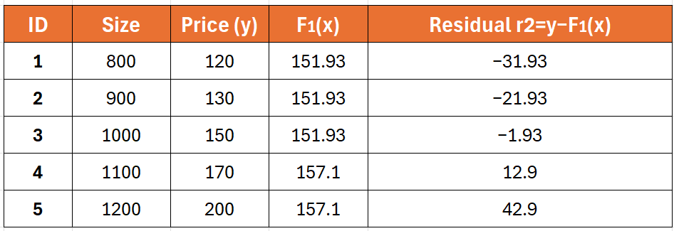
🧮 Candidate Split: Size < 1050

Divide data into two groups:

• Left group (Size < 1050): ID 1, 2, 3 → residuals [−31.93, −21.93, −1.93]

• Right group (Size ≥ 1050): ID 4, 5 → residuals [+12.9, +42.9]

🔢 Left Group Mean

\(\begin{aligned} \text{mean}(A) &= \frac{-31.93 + (-21.93) + (-1.93)}{3} \\[2ex] &= \frac{-55.79}{3} = -18.6 \end{aligned}\)

🔢 Right Group Mean

\(\begin{aligned} \text{mean}(B) &= \frac{12.9 + 42.9}{2} \\[2ex] &= \frac{55.8}{2} = 27.9 \end{aligned}\)

📌 Interpretation

So the second stump is:

\(h_2(x) = \begin{cases} -18.6 & \text{if } \text{Size} < 1050 \\[1ex] 27.9 & \text{otherwise} \end{cases}\)

🧮 SSE Check (to confirm best split)

Now compute squared errors relative to group means:

Left Group SSE

\(\begin{aligned} (-31.93 - (-18.6))^2 &= (-13.33)^2 = 177.7 \\[1.5ex] (-21.93 - (-18.6))^2 &= (-3.33)^2 = 11.1 \\[1.5ex] (-1.93 - (-18.6))^2 &= (16.67)^2 = 278.0 \\[2.5ex] \text{SSE}(A) &= 466.8 \end{aligned} \)

Right Group SSE

\(\begin{aligned} (12.9 - 27.9)^2 &= (-15)^2 = 225 \\[1.5ex] (42.9 - 27.9)^2 &= (15)^2 = 225 \\[2.5ex] \text{SSE}(B) &= 450 \\[1.5ex] \end{aligned} \)

\(\begin{aligned} \mathbf{\text{Total SSE}} &\mathbf{= 466.8 + 450 = 916.8} \end{aligned}\)

✅ Why This Split Was Chosen Again

• Among all candidate splits (Size thresholds, Beds thresholds), Size < 1050 still gave the lowest SSE.

• That’s why the second stump also used the same threshold, but with updated group means (−18.6 and 27.9).

---

🔁 Step 4 — Third Stump h₃(x)

Residuals r3 show the same sign pattern (IDs 1–3 negative, 4–5 positive).
So again, Size < 1050 remains the best split.

Each iteration reduces residual magnitude and total SSE.
Eventually, residuals shrink toward zero, meaning the model has learned the pattern.

---

🧠 Final Model Expression

\(F(x) = F_0 + \eta \cdot h_1(x) + \eta \cdot h_2(x) + \eta \cdot h_3(x) + \dots \)

---

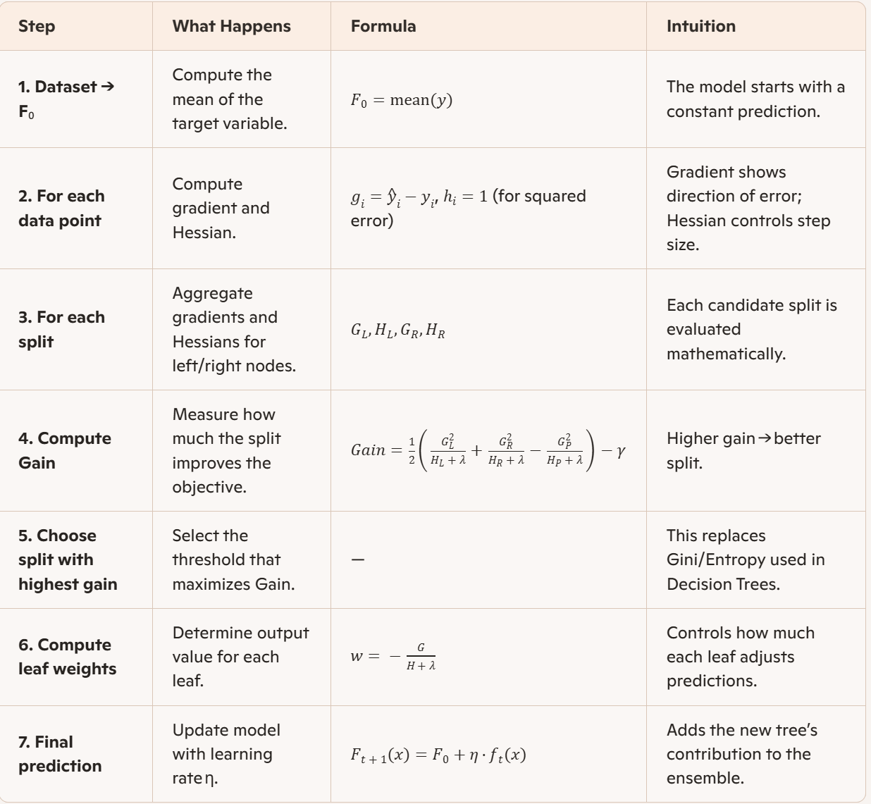
⚡ What Is XGBoost?

XGBoost (Extreme Gradient Boosting) is an advanced version of Gradient Boosting — it’s faster, more regularized, and mathematically refined.
Think of it as Gradient Boosting + Optimization + Regularization + Parallelization.

Here’s how it differs conceptually:

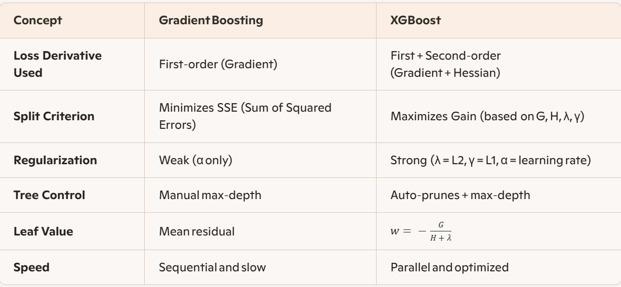
So, XGBoost improves Gradient Boosting by:

• Using both gradient and Hessian (Newton optimization).

• Adding L1 (γ) and L2 (λ) regularization to prevent overfitting.

• Computing gain to choose the best split mathematically.

• Allowing parallel tree building for speed.

---

🧩 Iteration 1 — Full Calculation Breakdown

1️⃣ Initial Setup

Step 0 — Base Model

• Initial prediction for all rows:

F0=mean(y)=154

\(F_0 = \text{mean}(y) = \frac{120 + 130 + 150 + 170 + 200}{5} = 154 \)

• Loss function: L=1/2(y−y^)2

• Gradient: g=y^−y

• Hessian: h=1 (for squared error)

• Regularization parameters:

  • λ=1 (L2)

  • γ=0 (L1 penalty, default off)

---

🧮 Iteration 2 — Full Calculation

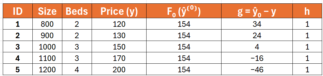
After Iteration 1, your predictions were:

---

Candidate Splits

Here G_I And G_r means Gradients Left(I) and Right (r) and Same goes H Hessians

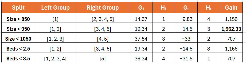
if you are wondering H Left and H Right for split point 850 is 1 and 4 when size is less than 850, the values get split accordingly

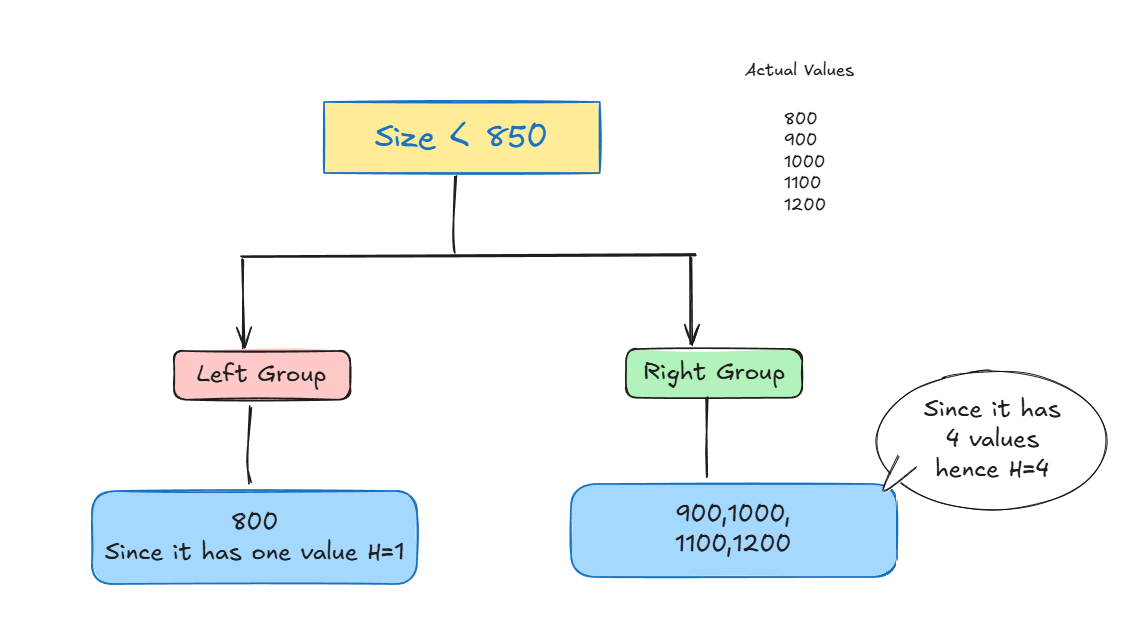
✅ Best split again: Size < 950 (Gain = 1962.33)

Since 950 turned out to be our best split, let's break down exactly how we got that gain value. Normally, we just look at all the midpoints and pick the one with the highest gain. Checking every single point by hand would take forever, so we’ll just walk through the math for 950. The exact same logic applies to all the other points anyway!

---

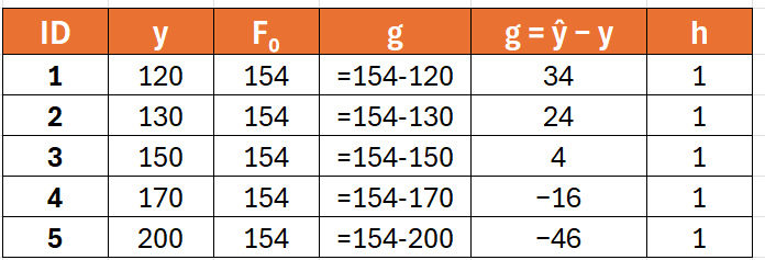
🧩 Step 1 —Recall Gradients & Hessians (Iteration 1)

From the base model F0=154:

---

🧩 Step 2 — Candidate Split at Size < 950

• Left group (ID’s, 1, 2):

G_L=34+24=58, H_L=1+1=2

• Right group (ID’s 3, 4, 5):

G_R=4+(−16)+(−46)=−58, H_R = 1+1+1=3

• Parent totals:

G_P = GL+GR =58+(−58)=0, H_P = 2+3=5

---

🧩 Step 3 — Gain Formula

\(\text{Gain} = \frac{1}{2} \left( \frac{G_L^2}{H_L + \lambda} + \frac{G_R^2}{H_R + \lambda} - \frac{G_P^2}{H_P + \lambda} \right) - \gamma \)

Parameters:

• λ=1 (L2 regularization)

• γ=0 (L1 penalty off)

---

🧩 Step 4 — Plugging Values

• Left term:

\(\frac{G_L^2}{H_L + \lambda} = \frac{58^2}{2 + 1} = \frac{3364}{3} = 1121.33 \)

• Right term:

\(\frac{G_R^2}{H_R + \lambda} = \frac{(-58)^2}{3 + 1} = \frac{3364}{4} = 841 \)

• Parent term:

\(\frac{G_P^2}{H_P + \lambda} = \frac{0^2}{5 + 1} = 0 \)

---

🧩 Step 5 — Final Gain

\(\text{Gain} = \frac{1}{2} (1121.33 + 841 - 0) = \frac{1962.33}{2} = 981.165 \)

Omit the ½ factor when presenting Gain, so they report the raw sum as 1962.33.

---

Now the split is fixed that is 950

🧩 Step 1 — Fix the Split

• The dataset is divided into two groups:

  • Left node (Size < 950): ID’s ——> 1, 2

  • Right node (Size ≥ 950): ID’s ——> 3, 4, 5

This becomes the first stump (tree with one split).

---

🧩 Step 2 — Compute Leaf Weights

Formula for leaf output: Leaf Weights

\(w = -\frac{G}{H} + \lambda \quad \text{with} \quad \lambda = 1 \)

\(\begin{align*} \text{Left node:} \quad & G_L = 58, \quad H_L = 2, \quad w_L = -\frac{58}{2 + 1} = -19.33 \\[1.5em] \text{Right node:} \quad & G_R = -58, \quad H_R = 3, \quad w_R = -\frac{-58}{3 + 1} = +14.5 \\[1.5em] \text{So the stump is:} \quad & h_1(x) = \begin{cases} -19.33 & \text{if } \text{Size} < 950 \\[0.8em] +14.5 & \text{otherwise} \end{cases} \end{align*} \)

G_L and G_R we got from previous steps

---

🧩 Step 3 — Update Predictions

Now we add the leaf weight to the base prediction F₀=154. Formula:

\(F_{1}(x) = F_{0}(x) + \eta \cdot h_{1}(x) \)

with learning rate η=1.

---

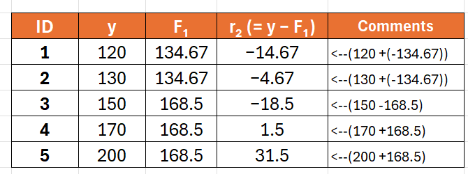
🧩 Step 4 — Compute New Residuals

Residuals after Iteration 

\(r_2 = y - F_1 \)

🔁 Iteration 3 (Conceptually)

You’d now compute new gradients g3=y^2−y and Hessians h3=1, then repeat the same gain and leaf‑weight process.
Each iteration refines predictions and reduces residuals further.

---

🧠 Intuitive Summary

• XGBoost starts like Gradient Boosting but adds mathematical rigor:

  • Gradient → direction of correction

  • Hessian → step size control

  • Regularization → stability

  • Gain → objective measure of split quality

• The model keeps building trees until residuals are minimized.

---